If you are not quite familiar with CNN, please view my previous blog for a better understanding.

BN-Inception

Related paper is: Batch Normalization: Accelerating Deep Network Training by Reducing Internal Covariate Shift, published on Mar. 2015.

Achievement

Improved the accuracy of ImageNet 1000 classification, the top-1 and top-5 error rate are 20.1% and 4.9% respectively.
Introduced the batch normalization, largely reduced the training time cost, for ImageNet classification network, by using batch normalization, can match the same performance as the previous network by only 7% of the training steps.
In some cases, time consuming dropout is not quite necessary for the network.
Personally, I think that this paper is very important and useful, but it’s not a good paper, because there’s a lot of ambiguous descriptions, some of them are quite contentious. I spent quite a lot of time on it, however, there’s still some details not that clear.
The related issue on this paper is based on references and my personal understanding, if you find any problem, correct me via any means you like please.

Internal Covariate Shift

In neural network’s training process, different input training instances’s data has different distributions, so that the later layers will have to continuously adapt to the new distribution. The input distribution on a learning system changes, it is said to experience covariate shift. You have to use small learning rate as well as initiate the network parameters carefully, the training speed will be quite slow.
More over, covariate shift’s bad effect will be more significant as the network structure getting deeper and deeper, because the shift can accumulate.
This paper refer to the change in the distributions of internal nodes of a deep network, in the course of training, as Internal Covariate Shift.

Batch normalization

Batch normalization is the most important and complex part of this paper. I think it’s better to introduce this part in Normalizations in neural networks.
As the paper illustrated, there’s a few tips for accelerating BN-Inception’s training:

• Increase learning rate.
• Remove Dropout.
• Reduce the L2 regularization.
• Accelerate the learning rate decay.
• Remove Local Response Normalization.
• Shuffle training examples more thoroughly.
• Reduce the photometric distortions.

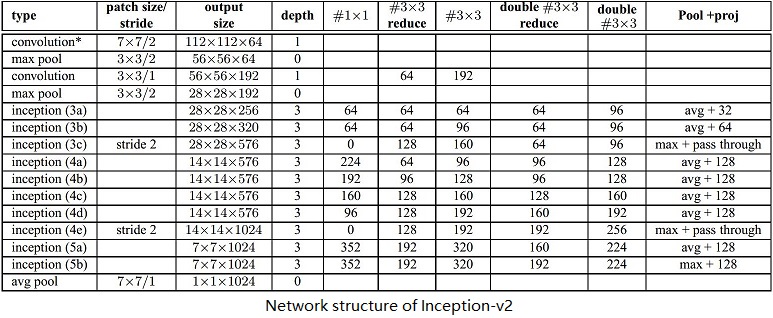
BN-Inception architecture

BN-Inception is derived from the GoogLeNet which is also called Inception net, please go to another blog to see the details on the GoogLeNet. The following content is the difference between the Inception-v2 and GoogLeNet.
During the forward training process, after the conv. op., the data will go through the batch normalization op. before passing the non-linear activation unit. And the batch normalization op. gets involved in the back propagation process as well.
During the inference process, the used mean for each neural is the average mean of all the batches for that neural and the variance is the unbiased estimate of the variances of all the batches.
The 5x5 conv. layers are replaced by two consecutive 3x3 layers. So, as I mentioned earlier, the depth of the Inception module grows to 3. This modification increases the number of parameters by 25% and the computational cost is increased by about 30%.
The number of 28x28 Inception modules is increased from 2 to 3.
Inside the Inception modules, the pooling method is not only max-pooling.
No across the board pooling layers between any two Inception modules, but stride-2 conv./pooling layers are employed before the filter concatenations in modules 3c, 4e.
The following figure is an illustration of BN-Inception architecture.

Inception Net

Related paper is: Rethinking the Inception Architecture for Computer Vision, published on Dec. 2015.

Achievement

Benchmark on ILSVRC 2012 classification challenge validation set, with a single model that has less than 25 million parameters, 5 billion multiply-adds op. (for a single inference), top-5 and top-1 error rate is 5.6% and 21.2%; with an ensemble of 4 models and multi-crop evaluation, reported 3.5% top-5 error rate and 17.3% top-1 error rate.

General Design Principles

Four architecture improve skills were raised, these skills are mostly based on the large-scale experimentation with various CNN architectural choices. The author issues to use these ideas judiciously!

• Avoid representational bottlenecks, especially early in the network. Down scale the input image and the feature maps gently.
• Higher dimensional representations are easier to process locally within a network. In a layer of the network, more activations per tile can make it easier to generate more disentangled features. More filters can accelerate training.
• Spatial aggregation can be done over lower dimensional embeddings without much or any loss in representational power. So, use dimension reduction generously, it wouldn’t affect too much on your performance if used properly.
• Balance the width and depth of the network. Make the computational budget balanced between the depth and the width of the your network.

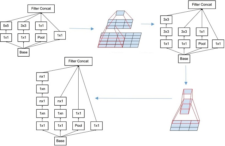
Factorizing Convolutions

Factorization the conv. kernel can reduce the computation. A 5x5 filter was factorized into two 3x3 consecutive conv. kernels. Inputs and outputs has the same size, but the computation load was reduced to (9+9)/25, it’s about 28% improvement. I spent sometime in figuring out how it actually works, if you also want to do so, one hint for you is that think about the influence of padding, Google’s architecture always use padding for inputs to get the same size outputs, but they never say!
Another inspiring change is the n by n conv. kernel can be factorized into a 1 by n kernel followed by a n by 1 kernel, they call this op. asymmetric convolutions. In the figure below, n equals 3. By doing so, the computation load is reduced to (3+3)/9 percent of without using it, it’s about 33%’s improvement.
The asymmetric conv. reminds me a problem about the high performance computing. For image data, usually we load the data into our DRAM either by row-wise (C style) or column-wise (Fortran style). If we store the data row-wise, we’d better to access the data row-wise and so do the colume-wise scenario in order to take advantage of L1 cache. Apparently, asymmetric conv. op. force us to access the data cross lines, it may cause the cache miss frequently if the image or feature map size is larger than the L1 cache size.
Actually, I have some concern here, because my intuition tells me that the factorization will depress the representation ability of the conv. operation. I’m not sure about it, but anyway, the result from the author seems quite promising.

Grid Size Reduction

Usually, grid size reduction is realized by pooling after a conv. op. and an activation, in order to avoid the representational bottleneck, usually, more conv. filter will be applied.
If there are n d by d feature maps to be conv. with k filters. To avoid representational bottleneck, if the pooling stride is 2, then usually, k = 2n.
Author think that by using inception module can reduce the computation complexity at the same time do not introduce the representation bottleneck.

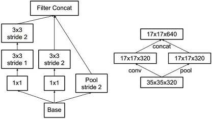
They implement grid reduction in a parallel way. First way uses three consecutive conv. op., the kernel size and conv. stride all are different; second way uses two consecutive conv. op.; the last way uses a pooling with stride 2. Then concatenate the results as the input of the next layer. The left image represents the operation progress of the inception module and the left represents the grid size reduction of the inception module of the same process.

Inception-v2

Inception-v2 factorize traditional 7x7 conv. into three consecutive 3x3 conv. with stride one. The architecture of Inception-v2 is shown in the figure below:

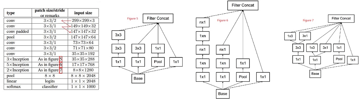
0-padding is used whenever necessary to maintain the grid size. Whole network is 42 layers deep, computational cost is 2.5 times higher than GoogLeNet.

Label Smoothing

Usually, in CNN, the label is a vector. If you have 3 class, the one-hot labels are [0, 0, 1] or [0, 1, 0] or [1, 0, 0], each of the vector stands for a class at the output layer.
Label smoothing, in my understanding, is to use a relatvely smooth vector to represent a ground truth label. Say [0, 0, 1] can be represented as [0.1, 0.1, 0.8].
According to the author:

First, it (using unsmoothed label) may result in over-fitting: if the model learns to assign full probability to the ground-truth label for each training example, it is not guaranteed to generalize. Second, it encourages the differences between the largest logit and all others to become large, and this, combined with the bounded gradient, reduces the ability of the model to adapt. Intuitively, this happens because the model becomes too confident about its predictions.

They claim that by using label smoothing, the top-1 and top-5 error rate are reduced by 0.2%.

ResNet

Related papers are:
Deep Residual Learning for Image Recognition, published on Dec. 2015 by Microsoft.
Indentity Mappings in Deep Residual Networks, published on Apr. 2016 by Microsoft.
Wide Residual Networks, published on Apr. 2016.
Most parts of this summary are based on the first paper.

Achievement

Deep residual net at ILSVRC2015 won the first place on image classification. The 152-layer depth resnet who has a lower complexity than VGG net achieved ensemble top-5 error rate is 3.57% (6 models), which is quite close to Inception-v3 multi-crop (144) multi-model(4) inference. This network also won the 1st place on: ImageNet detection, ImageNet localization, COCO detection, and COCO segmentation in ILSVRC & COCO 2015 competitions.

Residual Learning and Identity Mapping by Shortcuts

The key point of ResNet is residual learning and identity mapping by shortcuts.
The philosophy of residual learning I think is inspired by the traditional data representation and compression. As the network gets deeper and deeper, the training is more and more difficult. Residual learning is trying to solve this problem, the idea is: learning the differences or changes of the transformation is simpler than learning the transformation directly.
Usually, the input feature map will go through a conv. filter, a non-linear activation function and a pooling op. to get the output for the next layer. The conv. filter is trained by the back-propagation algorithm. As the network gets deeper, it is very hard for the conv. filter to converge. There’s many related research on it.
Residual learning, in my understanding, make an hypothesis that the input and the output has some kind of correlation. The way of doing the residual learning is to feed the input data directly to the output of the conv. op.’s output, add them together, then do the non-linear activation (ReLU) and pooling. The idea can be further generalized, the intermediate conv. op. can be multi-layer-conv., as shown as the figure below.

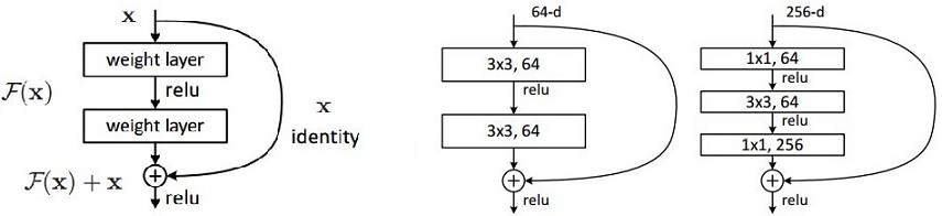
Padding op. is needed to keep the output has the same size of the input. The author claims that by using this block, the training speed for very deep network is faster than the counterpart without the block and also the accuracy is higher. The right two graph in above figure are two real residual learning block adopted by the ResNet.
Consider H(x) as an underlying mapping to be fit by a few stacked layers with x denoting the inputs to the first of these layers. Then hypothesize that the MLP can asymptotically approximate the residual function: H(x) - x. Rather than expect stacked layers to approximate H(x), we explicitly let these layers approximate a residual function F(x) := H(x) - x. The original function thus becomes F(x)+x. They call the forward-feeding op. identity mapping, and they also issue that identity mapping may not be the optimal but empirically, it’s better than zero mapping (no mapping as the convention).
The formula can be expressed by:
x and y are the input and output vectors of the layers. Function F(x, {Wi}) represents the residual mapping to be learned. At the above figure, F = W2 ( ReLU( W1( x ) ) ).
Above expression can be further extend to:
to express the multi-intermediate layer representation, the mapping can also adds some transformation, but the author claims that the identity mapping seems good enough.
I should say, the idea of residual learning is inspiring, but the process of the identity mapping looks like a very special case of inception module, I know there’s a lot of difference in the philosophy and the whole architecture, but I can still see the shadow of inception especially from the grid reduction part of inception.
One more comment is that I believe that residual learning may not suitable to shallow networks. Because for each residual block, they use identity mapping, so every time the output of the block can be seen as a kind of variation of the input, so if the network is not deep enough, the last layer feature extracted from the network may not be very repressive. The author issued in the article that they observed that the learned residual functions in general have small responses, intuitively, this statement makes me feel more confident to my judgment.

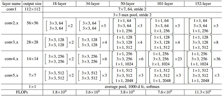
Architecture

A few version of ResNet for ImageNet classification was mentioned as the figure below:

Again, this post seems too long to maintain, the follow up paper will be summarized in another blog.

License