This blog summarizes techniques that have been revealed in publications in convolutional neural networks. The focus of this summary will be put on the terminologies and their influences. Related technics will not be explained in detail, for some algorithms, I may wrote other standalone articles to explain how they work.
Allow me to issue some abberviations, “conv.” means “convolution“, “op.” means operation, these two words appear too frequently.
LeNet-5
The related paper is : Gradient-Based Learning Applied to Document Recognition, released in 1998.
Structural Risk Minimization
This concept raised in two reference papers of this paper. In a gradient-based machine learning, there is:
(E_test:test set error) - (E_training: training set error) = (k: a constant) x ((h: a measure of effective capacity)/(P: size of training set)) ^ (α: a number between 0.5 and 1)
The gap between test error and training error will always decrease when the number of training samples increase. The increasing of the capacity h, training error will decrease, the gap will be larger.
To my understanding, this formula wants to issue, during the training process, the more data the better. But the capacity of the weights is not the wider the better, there should be some constrains on the weights’ parameter space in order to avoid overfitting and loss of the generalization of the network.
Regularization Function
In order to control the range of the network’s weights, they introduced the regularization function.
(E_bp: back propagation error) = (E_training: training set error) + (β: a constant) x (H(W: weights of the network): regularization function)
Use the regularization function as part of the back propagation error can limit the weights of the network, when minimizing the forward propagation error, the weights of the network also be limited. Regularization function can be quite simple sometimes, such as summing up all the weights’ value together and multiply with a constant.
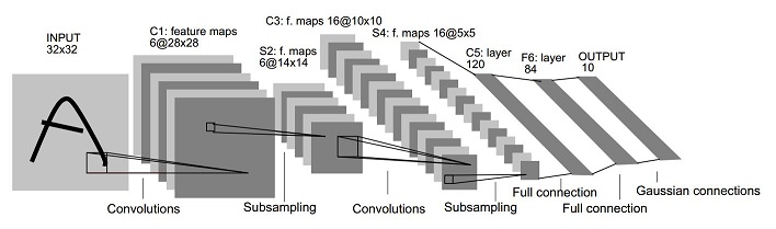
LeNet-5 architecture in detail
Not counting the input, LeNet-5 comprises 7 layers. Input image is 32x32 pixel image with a character on it. The largest character in database is at most 20x20 and the original image is 28x28. The reason to enlarge the size of the image is described as:
“It is desirable that potential distinctive features such as stroke end-points or corner can appear in the center of the receptive field of the highest-level feature detectors.”
Normalization for the input image is to set the background (white) to -0.1 and the foreground (black) to 1.175. By doing so, the mean of the input is roughly 0 and the variance is roughly 1, author claims that it can accelerates learning. Details will be illustrate in another blog: Normalizations in neural networks.
The first layer C1 is a convolutional layer with 6 output feature maps. Each unit in each feature map is connected to a 5x5 neighborhood in the input image, stride is one pixel, so the output size is 28x28 ((32: input_image_width/height)-(5: convolutio_kernel_width/height)+(1: compensition)). This layer contains 156 trainable parameters ((6: feature_map_number) x ((5x5: convolution_kernel_area) + (1: bias))) and 122,304 connections ((156: trainable_parameters) x (28x28: feature_map_size)).
The second layer S2 is a sub-sampling layer with 6 output feature maps of 14x14. Each unit in each feature map is connected to a 2x2 neighborhood in the corresponding feature map from the previous layer’s output. The four inputs to a unit in this layer are added, then multiplied by a trainable coefficient and added to a trainable bias. Let the result pass through a sigmoidal function. Totally 12 trainable parameters ((6: number_of_input_feature_map) x ((1: coefficient) + (1: bias))) and 5,880 connections ((14x14: output_feature_maps_size) x (6: output_feature_map_number) x (2x2: subsampling_kernel_size) + (1: bias))).
The third layer C3 is a convolutional layer with 16 output feature maps. Convolutional kernel size is 5x5, each unit in each feature map is connected to several 5x5 neighborhoods at identical locations in a subset of S2’s feature maps. The connection scheme is:
“First six C3 feature maps take inputs from every contiguous subsets of three feature maps in S2, the next six take input from every contiguous subset of four, the next three take input from some discontinuous subsets of four and finally the last one takes input from all S2 feature maps.”
Totally 16 feature maps. The reason of not connect every S2 feature map to every C3 feature map is that first, a non-complete connection scheme keeps the number of connections within reasonable bounds and second, it forces a break of symmetry in the network is that different feature maps are forced to extract different features because they get different sets of inputs.
C3 layer has 1,516 trainable parameters ((5x5x3x6:kernel_size x three_different_S2_feature_maps x six_output) + (5x5x4x9: kernel_size x four_different_S2_feature_maps x nine_output) + (5x5x6: kernel_size x six_different_S2_feature_maps) + (16:bias)) and 151,600 connections (1,516: trainable_parameters x 10x10: output_feature_map_size).
The fourth layer S4 is a sub-sampling layer with 16 5x5 feature maps. The way of sub-sampling is similar as C1 and S2, each unit in feature map is connected to a 2x2 neighborhood in the corresponding feature map in C3. This layer has 32 trainable parameters ((16: input_feature_map_number) x ((1: coefficient) + (1: bias))) and 2,000 connections ((5x5: output_feature_map_size) x ((2x2: sub-sampling_kernel_size) + (1: bias)) x (16: output_feature_map_number)).
Now I feel sorry to have describled this network structure…
The fifth layer C5 is also a convolutional layer with 120 1x1 output feature maps. Each unit is connected to a 5x5 neighborhood on all 16 of S4’s feature maps. This layer has 48120 trainable parameters (((5x5: kernel_size) x (16: input_feature_map_number) + (1: bias)) x (120: output_feature_map_number)). The reason of why this layer is named as convolutional layer instead of fully connected layer is that if the original input image is larger, the output feature map size is larger than 1x1.
The sixth layer F6 contains 84 uints is a fully connected layer with 10,164 trainable parameters (((120: input_feature_map_number) + (1: bias)) x (84: output_unit_number)). The reason of choosing 84 has some relationship with the desired object representation. In this paper, author illustrates that the target is to represent a stylized image of the corresponding character class drawn on a 7x12 (84) bitmap.
The last layer F7 is a fully connected layer with 10 outputs corresponding to 10 Arabic digits.
Unsupervised pretraining network for ImageNet object recognition
Related paper is : Building high-level features using large-scale unsupervised learning, published on 2012.
Achievement
Using unsupervised learning, an autoencoder, to extract high-level object features from large scale image dataset. Apply the unsupervised network as the initialization of the supervised learning network, training on 22000 classes ImageNet dataset, achieved 15.8% accuracy (70% relative improvement over the state-of-the-art at that time, the random guess accuracy is less than 0.005%).
Key techniques summary
Training dataset contains 10 million images from 10 million YouTube videos(each video contributes only one). Each example is a color image with size 200x200 pixels.
The model is a deep autoencoder with pooling and local contrast normalization. During training, asynchronous SGD is employed, training is distributed among a cluster with 16,000 cores for three days.
The idea of this unsupervised architecture comes from a neuroscientific conjecture that there exist highly class-specific neurons in the human brain named “grandmother neurons”, it means that a baby learns to group faces into one class because it has seen many of them without specific guidance.
Local contrast normalization
To normalize a layer’s outputs. For detail, please visit another blog: Normalizations in neural networks.
AlexNet
Related paper is : ImageNet Classification with Deep Convolutional Neural Networks, published on 2012.
Achievement
In ImageNet LSVRC-2010 contest, classify 1.2 million high-resolution images into 1000 different classes with top-1 and top-5 error rates of 37.5% and 17.0%; in ILSVRC-2012 competition a variant of this model achieved a top-5 test error rate of 15.3%.
Data set
ILSVRC-2010 uses subset of ImageNet data set with roughly 1,000 RGB images in each of 1,000 categories. Roughly 1.2 million training images, 50,000 validation images, and 150,000 testing images. Test set labels are available.
ILSVRC-2012 competition, the test set label is unavailable.
The images were down sampled to 256x256 pixels. For each image, first rescaled the image according to the shorter side, let the short side has the length of 256, then cropped out the central 256x256 patch from the rescaled image. Before feeding the images to the network, each pixel subtracts the mean pixel value of the whole data set.
Rectified Linear Unit(ReLU)
An activation function to replace sigmoid function or tanh function. The function is:
f(x: input_of_the_function) = max(0, x: input_of_the_function)
This activation function has the advantage of less time and space computation complexity. It is said that by using ReLU, training speed is several times faster than traditional saturation neuron models.
Local Response Normalization (LRN)
Raised to normalize the weights of the CNN. at the same layer. For detail, please visit another blog: Normalizations in neural networks.
The author claims that by using LRN, top-1 and top-5 error rates were reduced by 1.4% and 1.2% respectively for ImageNet classification, besides, for a four-layer CNN, they achieved a 13% test error rate without LRN and 11% with LRN.
Overlapping Pooling
A pooling layer can be thought of as consisting of a grid of pooling units spaced s pixels apart, each summarizing a neighborhood of size z x z centered at the location of the pooling unit. If we set s = z, we obtain traditional local pooling as commonly employed in CNNs. If we set s < z, we obtain overlapping pooling.
In AlexNet, they set s = 2, z = 3. This pooling scheme is adopted throughout the network, and comparing to s = 2, z = 2, this scheme reduces the top-1 and top-5 error rates by 0.4% and 0.3% respectively.
They also issue that overlapping pooling network is a little bit more difficult to overfit.
AlexNet Architecture
The network contains five convolutional and three fully-connected layers.(removing any convolutional layer resulted in inferior performance)
The first convolutional layer filters the 224x224x3 input image with 96 kernels of size 11x11x3 with a stride of 4 pixels. The second convolutional layer takes as input the (response-normalized and pooled) output of the first convolutional layer and filters it with 256 kernels of size 5x5x48. The third, forth, and fifth convolutional layers are connected to one another without any intervening pooling or normalization layers. The third convolutional layer has 384 kernels of size 3x3x256 connected to the (normalized, pooled) outputs of the second convolutional layer. The fourth convolutonal layer has 384 kernels of size 3x3x192, and the fifth convolutional layer has 256 kernels of size 3x3x192. The fully-connected layers have 4096 neurons each.
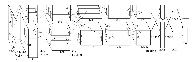
Ironically, what has been described above doesn’t match the paper’s figure. If anybody see this, please be noted that there’s something wrong with that paper.
I tried to analysis all the architecture parameters in that paper and found that almost all the given value cannot be understood by conventional method.
If you are interested, please to go this page (released by Stanford), and ctrl + f to search 224 in that page, there’s another illustration on AlexNet. An additional proof of padding can be found at tensorflow‘s AlexNet implementation.
Other Performance Related Techniques
Data Augmentation is adopted, first is a random crop 224x224x3 image from a 256x256x3 image, this method increases the data set by a factor of 2048, second thing is to apply a RGB intensities altering based on PCA (Principle Component Analysis), the idea is to enhance principle property (with randomness) of the image. This method reduces the top-1 error rate by over 1%.
Drop out is adopted.During the training, setting to zero the output of each hidden neuron with probability 0.5, by changing the connectivity of the network to reduce the overfitting problem. The other side of drop out is that it almost doubled the iterations required to converge.
Backpropagation parameters, SGD weight decay is 0.0005, batch size is 128, momentum is 0.9, initial learning rate is 0.01, reduce three time (by the factor of 0.1, when the validation result doesn’t change, manually adjust the learning rate) before training finished, they trained the network about 90 cycles over 1.2 million images.
Initialization, weights in each layer was initialized by zero-mean Gaussian distribution with standard deviation 0.01. Biases besides the first convolutional layer (initialized by 0) are initialized by a constant 1, it can help to accelerate the early stages of learning by providing ReLUs with positive inputs.
GoogLeNet
Related paper is: Going deeper with convolutions, published in 2014.
Achievements
ILSVRC 2014 object recognition top-5 error of 6.67%, ranking the first place.
Input Data and Data Augmentation
Data set is ILSVRC 2014 challenge data set, it contains 1,000 categories. 1.2 million images for training, 50,000 for validation and 100,000 for testing.
For each image, resize the image according to the short edge with the length of 256, 288, 320, 352. Then, take the left ,center and right square of these resized images(top, center and down for portrait images). For each square, take the 4 corners and center 224x224 crop as well as the square resized to 224x224 and their mirrored version. So, each image in the data set will generate 4x3x6x2 = 144 training images.
So the input image of the network is a 224x224x3 image. Extract mean before feeding the training image to the network.
Inception Module
Inception architecture is a very interesting design. The conventional CNN usually convolute on a fixed size over the whole image. Inception architecture has a multi-scale convolutional structure. Different convolutional kernel sizes are adopted by the inception unit. In the article, they use 1x1 convolution kernel, 3x3 convolution kernel and 5x5 conventional kernel to convolute over feature maps, generating the same size output feature maps, then concatenate the outputs as the input of the next layer.
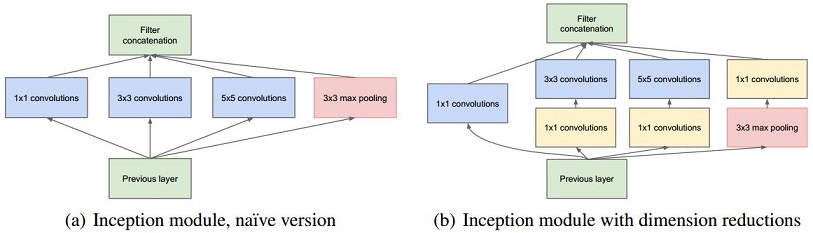
The 1x1 convolution has the effect of dimension reduction. Let’s say you have 56x56x64 feature maps, and you think 64 is too large, then you maybe consider to use 32 1x1x64 filters to convolute over your feature maps, the output will be 56x56x32, the dimension of the output is reduced by a factor of 2. If you still think it’s odd, think about RGB to gray scale image conversion(another name is RGB to Y), the difference is that the RGB to gray conversion’s filter is fixed (Gray = 0.2989 x R + 0.5870 x G + 0.1140 x B), but in the CNN, dimension reduction’s filter will be adjusted during the training process. And of course there will be some information loss during the reduction.
GoogLeNet Architecture
GoogLeNet, comparing with the above architectures, is quite complex.
The first convolutional layer is a layer with 64 output feature maps. Convolution kernel size is 7x7x3 with step 2. Input image is 224x224x3 (with padding 3 I believe), the output feature is 112x112x64. Then ReLU and max pooling by 3x3 kernel with step 2, now the output feature map size is 56x56x64. Then do the local response normalization.
The second convolutional layer has a simplied inception architecture. There’s 64 1x1x64 convolution operations who generate 64 feature maps from the previous layer’s output before the 192 3x3x64(with step 2) convolutions take effect. Then again do the ReLU and local response normalization. Afterwards, there’s a 3x3 max pooling with step 2. Now, the output is 192 28x28 feature maps.
The third layer contains a complete inception module. The previous layer’s output is 28x28x192 and there will be 4 branches after that, the first branch uses 64 1x1 convolution kernels and ReLU, generating 28x28x64 feature map; the second branch uses 96 1x1 convolution kernels as the dimension reduction(with ReLU) before 128x3x3 convolution operation, generating 128x28x28 feature map; the third branch uses 16 1x1 conv. kernel as reduction(with ReLU) of 32x5x5 conv. operation, generating 32x28x28 feature map; the forth branch contains 3x3 max pooling layer and a 1x1 conv. operation, generating 32x28x28 feature maps. Concatenate the generated feature maps, you get a 256x28x28 feature map.
The so called forth layer is nothing but another inception module. Input is the output of the previous layer, 28x28x256. Still four branches, 1x1x128 and ReLU, 1x1x128 as reduce before 3x3x192 conv. op., 1x1x32 as reduce before 5x5x96 conv. op., 3x3 max pooling with padding 1 before 1x1x64. The output for the four branches are respectively: 28x28x128, 28x28x192, 28x28x96 and 28x28x64. The total result is 28x28x480.
The following layers has quite similar structure. The following two figures from the paper illustrates the whole network. I don’t think you can see the structure clearly here, so find that paper, page 6 and page 7.
About the “depth” in the first figure, it represents a layer’s depth, for Inception module, before conv. op., there are 1x1 conv. reduction op. so that the depth is 2, maxpooling depth is 0 and normal conv.’s depth is 1. In the next version of inception net, you can see the variations of inception module has a depth of 3.
For the second figure, there’s some intermediate output, that’s fine, according to the paper, some intermediate layer’s output also provides acceptable accuracy with less complexity of the overall structure.
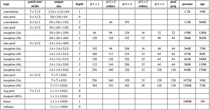
Figure1: GoogLeNet in detail
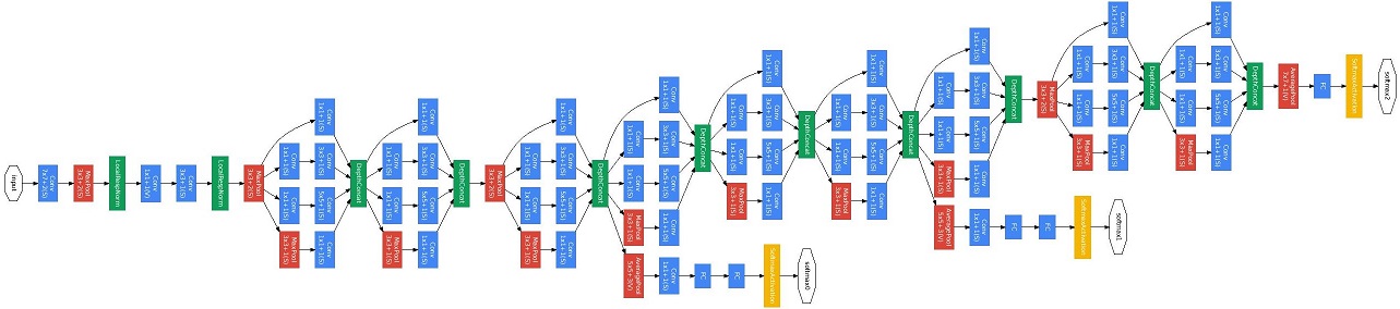
Figure2: GoogLeNet graph
Since this blog is too long to maintain and indexing, I’d better to start another blog for the papers afterwards.
License
The content of this blog itself is licensed under the Creative Commons Attribution 4.0 International License.

The containing source code (if applicable) and the source code used to format and display that content is licensed under the Apache License 2.0.
Copyright [2016] [yeephycho]
Licensed under the Apache License, Version 2.0 (the “License”);
you may not use this file except in compliance with the License.
You may obtain a copy of the License at
Apache License 2.0
Unless required by applicable law or agreed to in writing, software
distributed under the License is distributed on an “AS IS” BASIS,
WITHOUT WARRANTIES OR CONDITIONS OF ANY KIND, either
express or implied. See the License for the specific language
governing permissions and limitations under the License.